Core Loss Calculation
The article below provides a step-by-step method to calculate losses generated by powder cores under certain conditions. To compare core performance of all five Magnetics powder core materials, download our Curve Fit Equation tool or view our list of Powder Core Calculations.
Core loss is generated by the changing magnetic flux field within a material, since no magnetic materials exhibit perfectly efficient magnetic response. Core loss density (PL) is a function of half of the AC flux swing (½ B=Bpk) and frequency (f). It can be approximated from core loss charts or the curve fit loss equation:

where a, b, c are constants determined from curve fitting, and Bpk is defined as half of the AC flux swing:

Units typically used are (mW/cm3) for PL, Tesla (T) for Bpk, and (kHz) for f. The task of core loss calculation is to determine Bpk from known design parameters.
Method 1 – Determine Bpk from DC Magnetization Curve. Bpk= f(H)
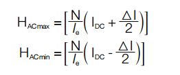
Flux density (B) is a non-linear function of magnetizing field (H), which in turn is a function of winding number of turns (N), current (I), and magnetic path length (le). The value of Bpk can typically be determined by first calculating H at each AC extreme:

Units typically used are (A•T/cm) for H.
From HAC max, HAC min, and the BH curve or equation (listed in Magnetics Powder Core Catalog pgs. 106-126), BAC max, BAC min and therefore Bpk can be determined.

Example 1 – AC current is 10% of DC current:
Approximate the core loss of an inductor with 20 turns wound on Kool Mμ p/n 77894A7 (60μ, le=6.35cm, Ae=0.654 cm2, AL=75 nH/T2). Inductor current is 20 Amps DC with ripple of 2 Amps peak-peak at 100kHz.
1.) Calculate H and determine B from BH curve or curve fit equation:

2.) Determine Core Loss density from chart (catalog pg. 63) or calculate from loss equation (catalog pg. 104):

3.) Calculate core loss:

Example 2 – AC current is 40% of DC current:
Approximate the core loss for the same 20-turn inductor, with same inductor current of 20 Amps DC but ripple of 8 Amps peakpeak at 100kHz.
1.) Calculate H and determine B from BH curve fit equation:

2.) Determine Core Loss density from chart or calculate from loss equation:

3.) Calculate core loss:

Example 3 – pure AC, no DC:
Approximate the core loss for the same 20-turn inductor, now with 0 Amps DC and 8 Amps peak-peak at 100kHz.
1.) Calculate H and determine B from BH curve fit equation:

2.) Determine Core Loss density from chart or calculate from loss equation:

3.) Calculate core loss:

Plotted below are the operating ranges for each of the three examples.
Note the significant influence of DC bias on core loss, comparing Example 3 with Example 2. Lower permeability results in less Bpk, even if the current ripple is the same. This effect can be achieved with DC bias, or by selecting a lower permeability material.

Method 2, For small ▲H, approximate Bpk from effective perm with DC bias. Bpk = f(μe, ▲H)
The instantaneous slope of the BH curve is defined as the absolute permeability, which is the product of permeability of free space (μ0=4π x10-7) and the material permeability (μ), which varies along the BH curve. For small AC, this slope can be modeled as a constant throughout AC excitation, with μ approximating the effective perm at DC bias (μe):

The effective perm with DC bias is more commonly written in terms of % of initial perm and can be obtained from the DC bias curve or curve fit equation:

▲H is multiplied by 100/4π because H units here are Oersteds and B units are Tesla.
Reworking Example 1 (20 Amps DC, 2 Amps pk-pk)
.JPG)
Reworking Example 2 (20 Amps DC, 8 Amps pk-pk)

Reworking Example 3 (0 Amps DC, 8 Amps pk-pk)

Method 3, for small ▲H, determine Bpk from biased inductance. Bpk=f(L,I)
B can be rewritten in terms of inductance by considering Faraday’s equation and its effect on inductor current:

Where L varies non-linearly with I. For small AC, L can be assumed constant throughout AC excitation and is approximated by the biased inductance (LDC).

Another way of looking at this is by rewriting the relationship between B and L as:

Substituting (dH/dI) with (N/le) and A with Ae:

Where L varies non-linearly with H. For small AC, the slope of the BH curve is assumed constant through AC excitation, and L is approximated by the biased inductance (LDC).

Reworking Example 1:

Reworking Example 2:

Reworking Example 3:

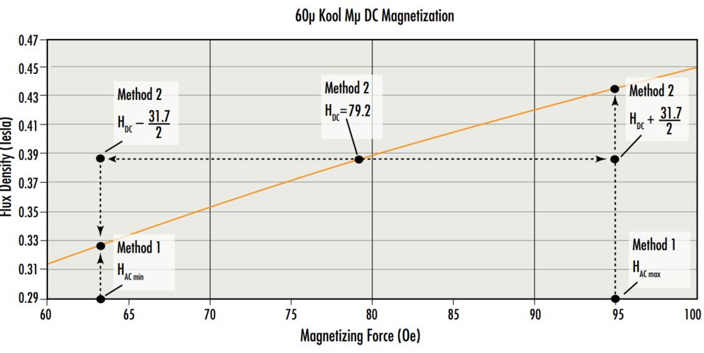
The plot below illustrates the difference between Method 1 and Method 2:
